
In the previous two sections we learned how to draw some graphs and how to look for correlations between factors in the Bearable data export.
Today we will look into how we can correlate your mood with factors.
Split details into factors
This should look familiar:
library(tidyverse)

data <- read.csv("./data/latest.csv")
df <- data %>% filter(data$category == "Mood" | data$category == "Factors" )

for (v in 1:nrow(df)) {
  curr_date <- df$date[v]
  same_dates <- df %>% filter(df$date == curr_date)
  df$detail[v] <- paste(same_dates$detail, collapse = ' | ')
}

df <- df %>% distinct(date, .keep_all = TRUE)

for (v in 1:nrow(df)) {
  factors <- str_split(df$detail[v], pattern="\ \\|\ ", simplify=TRUE)
  for (f in factors) {
    if (f == "|" || f == "") {
      next
    }

    if (!(f %in% colnames(df))) {
      df[f] <- as.logical(c(FALSE)*nrow(df))
    }

    df[v, f] <- TRUE
  }
}

drop <- c("detail", "notes", "time.of.day", "category", "weekday", "day")
df <- df[,!(names(df) %in% drop)]
Let’s average mood by date and write it back to the dataframe:
mood <- data %>% filter(data$category == "Mood")
mood$rating.amount <- as.numeric(mood$rating.amount)
mood <- mood %>% group_by(date) %>%
  summarise_at(vars(rating.amount), list(rating.amount = mean))

for (i in 1:nrow(df)) {
  df$rating.amount[i] <- mood$rating.amount[mood$date == df$date[i]][1]
}
df$rating.amount <- as.numeric(df$rating.amount)
We can drop the date field now:
drop <- c("date")
df <- df[,!(names(df) %in% drop)]
We only care about strong correlations (> 0.5):
corr <- cor(df)[, "rating.amount"] %>% sort
corr <- corr[abs(corr) > 0.5]
Plot the result:
c <- data.frame(name=names(corr), value=corr)
ggplot(c, aes(y=value, x=name, fill=value)) +
  scale_y_continuous(limits = c(-1,1)) +
  geom_bar(stat="identity")
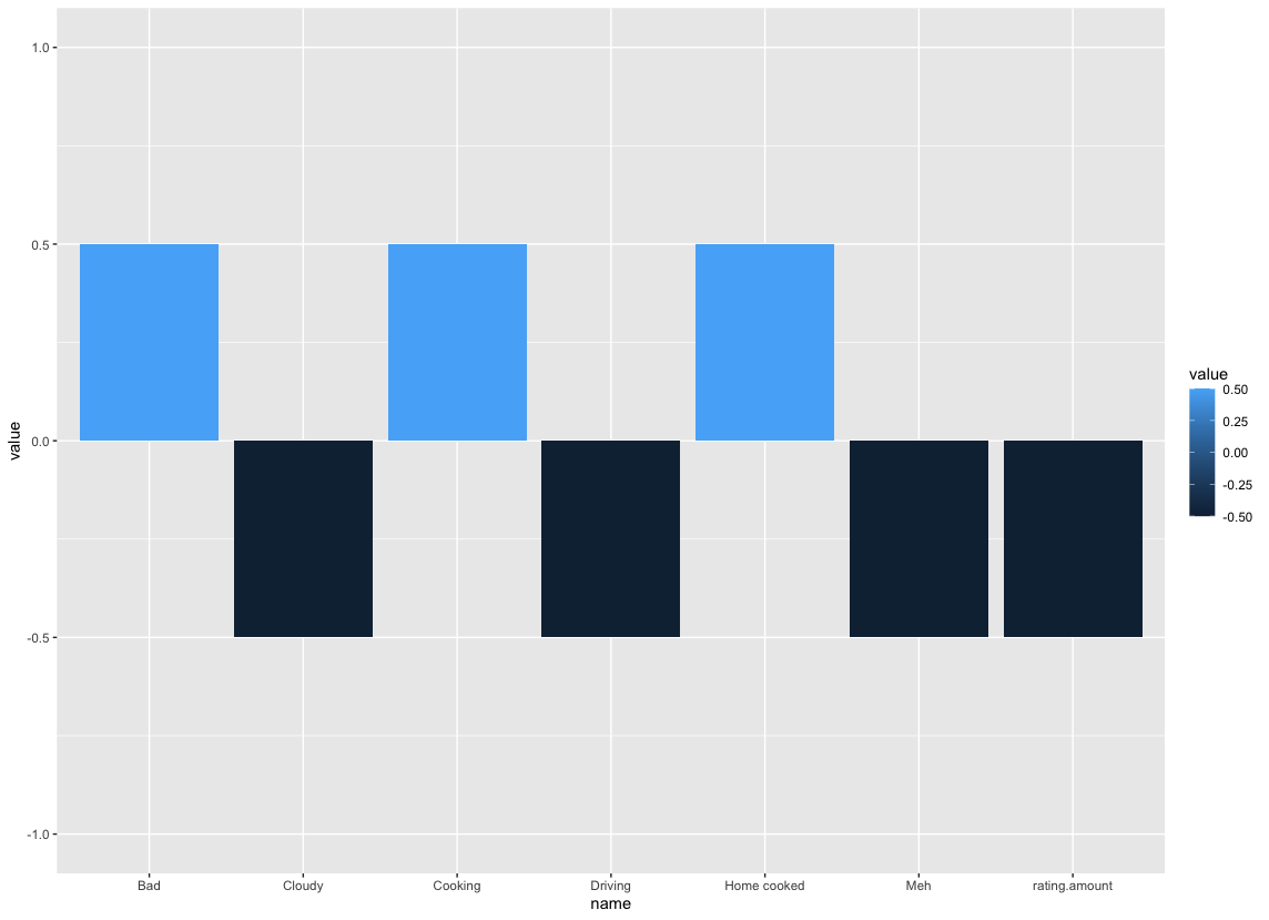 (The data is generated, for privacy reasons.)
Looking for statistically significant influencing factors
A strong correlation is a good indicator that something is statistically significant, but it’s best to make sure.
Let’s choose a factor and build a linear model:
> summary(glm(df$rating.amount ~ df$Cloudy))

Call:
glm(formula = df$rating.amount ~ df$Cloudy)

Deviance Residuals:
     Min        1Q    Median        3Q       Max
-0.49468  -0.33611  -0.09468  -0.03611   1.15532

Coefficients:
              Estimate Std. Error t value Pr(>|t|)
(Intercept)     6.5361     0.2742  23.836 5.82e-08 ***
df$CloudyTRUE  -1.4414     0.3679  -3.918  0.00576 **
---
Signif. codes:  0 ‘***’ 0.001 ‘**’ 0.01 ‘*’ 0.05 ‘.’ 0.1 ‘ ’ 1

(Dispersion parameter for gaussian family taken to be 0.3007786)

    Null deviance: 6.7226  on 8  degrees of freedom
Residual deviance: 2.1055  on 7  degrees of freedom
AIC: 18.467

Number of Fisher Scoring iterations: 2
The two stars (**) show that our model is statistically significant (p < 0.01).
